Column and line chart in excel
Let us create to understand how it works and how to create with an example. For Example we have 4 values A B C.

Microsoft Excel Dashboard Excel Tutorials Microsoft Excel Microsoft Excel Tutorial
For information on column charts and when they should be used see Available chart types in Office.
. Click the column chart to activate the Chart Tools and then click Design Add Chart Element Trendline Moving Average. Right-click the chart Select Data Edit the Horizontal category Axis Labels change. Create Area Chart in Excel.
Pie Chart in Excel is used for showing the completion or main contribution of different segments out of 100. Steps to Insert a Static Vertical Line a Chart. Excel Funnel Chart.
Change the chart type of the last three series to Scatter with Straight Lines and Markers and UNCHECK the Secondary Axis checkbox for all XY series. Pie Chart in Excel. It will create a Line and Stacked Column Chart with dummy data as shown in the below screenshot.
Insert a column chart. With the pivot chart selected click the Design tab on the Excel Ribbon. Click on the chart youve just created to activate the Chart Tools tabs on the Excel ribbon go to the Design tab Chart Design in Excel 365 and click the Select Data button.
Make sure your labels are formatted as text or they will be added to the chart as a third set of bars. Select the table and insert a Combo Chart. Only if you have numeric labels empty cell A1 before you create the column chart.
Open excel and create a data table as below. We can see that the Sales of yogurt has risen. Excel Chart Types Excel Chart Types.
Lets consider making a stacked column chart in Excel. The tutorial walks through adding an Average calculated column to the data set and graph. You may also learn more about Excel from the following articles.
It can be used only for trend projection pulse data projections only. In this example I set both sliders to 0 which resulted in no overlap and a slight gap. Cons of Line Chart in Excel.
Follow the below steps to show percentages in stacked column chart In Excel. If you are using Excel 2010 or earlier versions please click the chart to activate the Chart Tools and then click Layout Trendline Two Period Moving Average. Line Chart with a combination of Column Chart gives the best view in excel.
If you are just looking to visually hide the column but keep the data in the chart I recommend changing the column width to a small value like 01 to shrink it to near invisible. After creating the chart you can enter the text Year into cell A1 if. Since I have used the Excel Tables I get structured data to use in the formulaThis formula will enter 1 in the cell of the supporting column when it finds the max value in the Sales column.
If we make changes to the spreadsheet the column will also change. Go to Insert Column or Bar Chart Select Stacked Column Chart. To modify the axis so the Year and Month labels are nested.
A clustered column chart in Excel is a column chart that represents data virtually in vertical columns in series. Please follow these steps. Always enable the data labels so that the counts can be seen easily.
Click OK to accept the recommended chart layout a Clustered Column chart. Next we changed the Color to. Here is the step-by-step guide to creating a clustered column chart using Excel data on Power BI.
Excel Pie Chart Table of Contents Pie Chart in Excel. Enter a new column beside your quantity column and name it Ver Line. Though these charts are very simple to make these charts are also complex to see visually.
First click on the Line and Stacked Column Chart under the Visualization section. Format Line and Clustered Column Chart General Settings. This article is a guide to Line Chart Examples in Excel.
Use this General Section to Change the X Y position Width and height of a Line and Clustered Column Chart. A pivot chart is added to the worksheet showing the 2 years of data. It is another column chart type allowing us to present data in percentage.
Excel centers these axis titles along the sides of the chart. Convert to a combination chart as we did above for the column-line chart. Learn how to add a horizontal line to a column bar chart in Excel.
You can create a combination chart in Excel but its cumbersome and takes several steps. Right-click on any series and select Change Series Chart Type from the pop-up menu. Add a Chart Title.
First we used the Position drop-down to change the legend position to Top Center. Here you have a data table with monthly sales quantity and you need to create a line chart and insert a vertical line in it. Creating a Line Column Combination Chart in Excel.
The Line Chart is especially useful in displaying trends and can effectively plot single or multiple data series. Stacked column chart. To change the chart type please use same steps which I have used in the previous method.
The clustered chart is very simple and easy to use. What is the Excel Chart Wizard. Markerscircles squares triangles or other shapes which mark the data pointsare optional.
We discuss the top 7 line chart types practical examples and a downloadable Excel template. Now you have to change the chart type of target bar from Column Chart to Line Chart With Markers. In the chart click the Forecast data series column.
How to Make Pie Chart in Excel. Go To Insert Charts Column Charts 2D Clustered Column Chart. Step 5 Adjust the Series Overlap and Gap Width.
By way of example lets substitute 4000 for 1400 in yogurt sales. Select columns BJ and insert a line chart do not include column A. Using the plus icon Excel 2013 or the Chart Tools Layout tab Axis Titles control Excel 20072010 add axis titles to the two vertical axes.
For creating a Clustered column chart we have to prepare data or we can download it from the browser. In the Select Data Source window click the Add button. This helps in the presentation a lot.
Select the entire data table. Create Stacked Column Chart in excel. It is like each value represents the portion of the Slice from the total complete Pie.
Pie Column Line Bar Area and Scatter. Youll get a chart like below. Now enter a value 100 for Jan in Ver Line column.
Select your data and then click on the Insert Tab Column Chart 2-D Column. Column charts are useful for showing data changes over a period of time or for illustrating comparisons among items. Things to Remember about Line Chart in Excel.
In column charts categories are typically organized along the horizontal axis and values along the vertical axis. For example if there is a single category with multiple series to. Or click the Chart Filters button on the right of the graph and then click the Select Data link at the bottom.
Add Data labels to the. Next we are adding Profit to Line Values section to convert it into the Line and Stacked Column Chart. To create a column chart in excel for your data table.
In the Format ribbon click Format SelectionIn the Series Options adjust the Series Overlap and Gap Width sliders so that the Forecast data series does not overlap with the stacked column. Format Legend of a Line and Clustered Column Chart in Power BI. Create a Line and Stacked Column Chart in Power BI Approach 2.
The default Excel chart legends can be awkward and time consuming to read when you have more than 2 series in your chart. At the left click Add Chart Element. Select the entire table including the supporting column and insert a combo chart.
By doing this Excel does not recognize the numbers in column A as a data series and automatically places these numbers on the horizontal category axis. Theres no title on the chart so follow these steps to add a title.

How To Create A Graph In Excel 12 Steps With Pictures Wikihow Excel Bar Graphs Graphing

Adding Up Down Bars To A Line Chart Chart Excel Bar Chart

Stacked Column Chart With Optional Trendline E90e50fx

Multiple Width Overlapping Column Chart Peltier Tech Blog Data Visualization Chart Multiple

Ablebits Com How To Make A Chart Graph In Excel And Save It As Template 869b909f Resumesample Resumefor Charts And Graphs Chart Graphing

Chart Collection Chart Bar Chart Over The Years

Horizontal Line Behind Columns In An Excel Chart Excel Chart Create A Chart

Stacked Column Chart Uneven Baseline Example Chart Bar Chart Excel

Excel Actual Vs Target Multi Type Charts With Subcategory Axis And Broken Line Graph Pakaccountants Com Excel Tutorials Excel Graphing

How To Add A Secondary Axis In Excel Charts Easy Guide Trump Excel Excel Chart Tool Chart

Multiple Width Overlapping Column Chart Peltier Tech Blog Chart Powerpoint Charts Data Visualization

Side By Side Bar Chart Combined With Line Chart Welcome To Vizartpandey Bar Chart Chart Line Chart
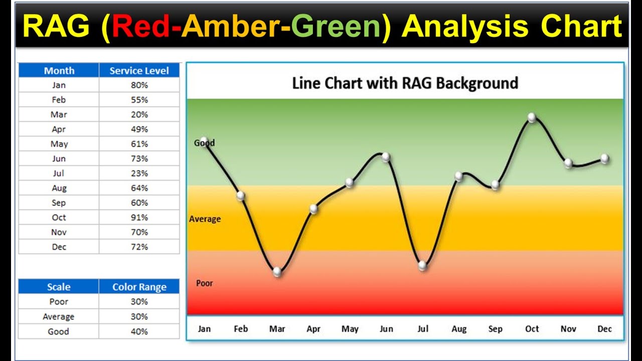
Rag Red Amber Green Analysis Chart In Excel Line Chart With Rag Background Youtube Excel Analysis Line Chart

Add Vertical Date Line Excel Chart Myexcelonline Line Vertical Excel

How To Add An Average Line To Column Chart In Excel 2010 Excel How To Excel Microsoft Excel Tutorial Excel Tutorials

Excel Charts Excel Microsoft Excel Computer Lab Lessons

Graphs And Charts Vertical Bar Chart Column Chart Serial Line Chart Line Graph Scatter Plot Ring Chart Donut Chart Pie Chart Dashboard Design Bar Chart